Part 2 — Building the Model · From Physics to 31,960 Labelled Picks
Part 1 ended at an architecture with a band most systems do not need: a development stage that exists only because the labels did not.
This post is that band, plus the module it feeds. It is where most of the work went.
Where the data actually comes from
The source is not photographs of individual apples. It is partial views of trees, photographed in an orchard.
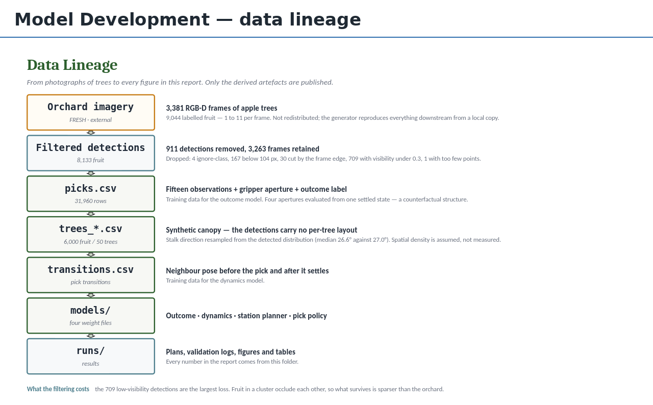
Figure 1. From photographs of trees to every figure in the report. Only derived artefacts are published — the generator reproduces everything downstream from a local copy.
The FRESH dataset carries 3,381 RGB-D frames with between one and eleven labelled apples in each, for 9,044 in total. Position, size, and the direction the stem points. That last field is why this dataset and not another: reconstructing a physical scene requires knowing which way the fruit hangs, and few public datasets provide it.
Not all 9,044 can be used. A detection has to carry a reliable diameter and stem direction before a scene can be built around it, and 911 of them do not.
| Stage | Remaining | Removed | Reason |
|---|---|---|---|
| Raw labels | 9,044 | ||
| Ignore class removed | 9,040 | 4 | Withheld by the annotator |
| Bounding box min side ≥ 104 px | 8,873 | 167 | Too distant for a stable diameter |
| Not truncated at the frame edge | 8,843 | 30 | Part of the shape outside the image |
| Visibility ≥ 0.3 | 8,134 | 709 | Occluded by leaves or other fruit |
| Point cloud ≥ 200 points | 8,133 | 1 | No 3D shape could be built |
Table 1. Filtering the detections. 8,133 survive.
The visibility rule is the one to keep in mind, and not only because it removes the most. Fruit growing in a cluster occlude one another, so they tend to be dropped together. What survives is therefore sparser than the orchard was, and any figure that depends on how crowded a tree is inherits that bias. Part 3 comes back to it.
A scene per fruit
The obvious way to build a simulator is to make one scene and swap the apple. That does not work here, and the reason is the gripper.
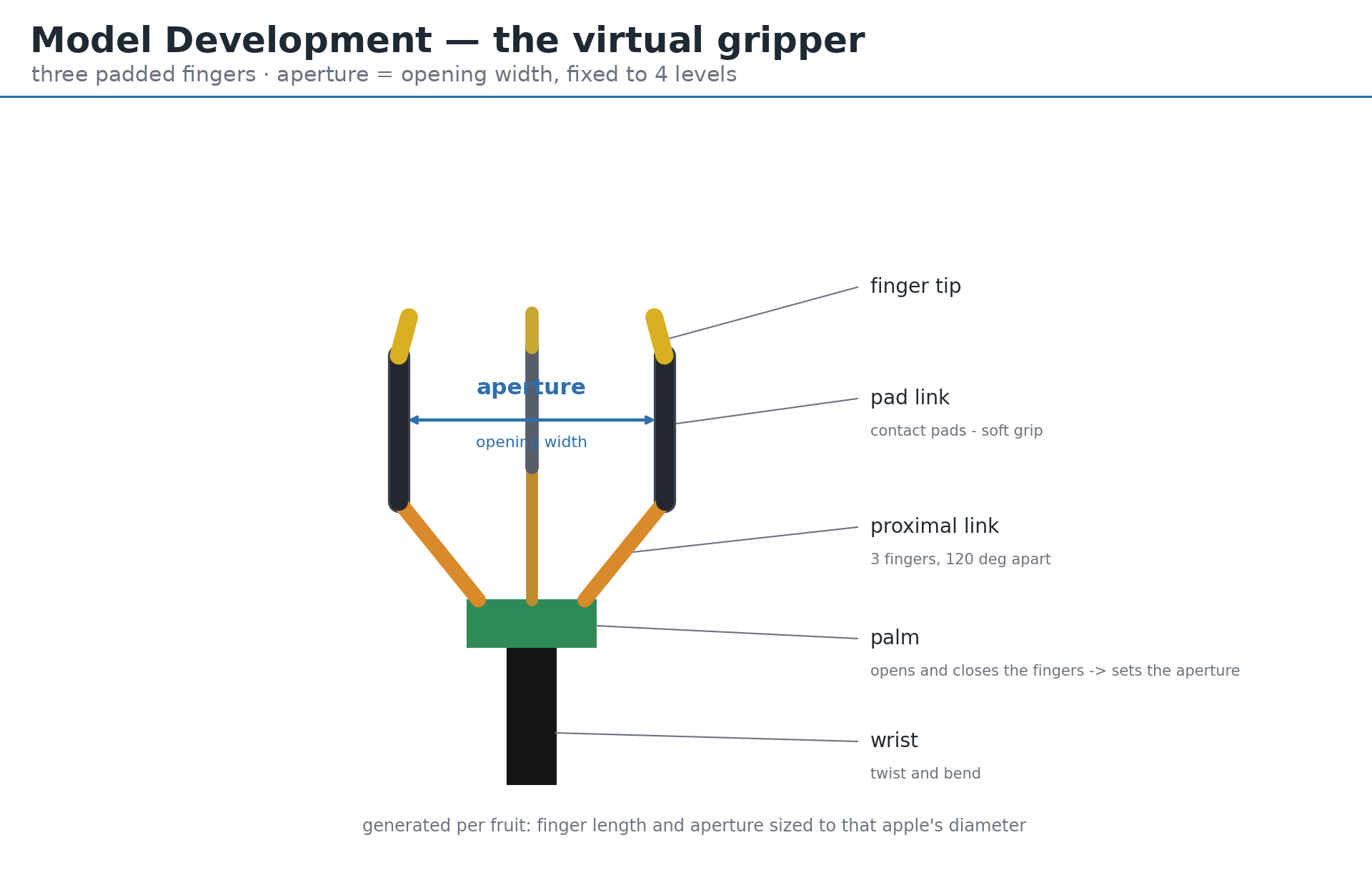
Figure 2. Three padded fingers, 120 degrees apart, closing onto a palm. The gripper is generated per fruit: finger length and aperture sized to that apple’s diameter.
Three padded fingers, 120 degrees apart, closing onto a palm. The aperture is how wide they open, and every other dimension follows from it: finger length, pad spacing, basket depth. The aperture in turn is set in proportion to the fruit’s estimated diameter.
So a 52 mm apple and an 84 mm apple are not the same problem with a different sphere in the middle. They are gripped by different hardware. A fixed scene cannot represent that, which is why the generator assembles a fresh MJCF scene for each of the 8,133 detections.
Three details in that scene matter more than they look.
The stalk is five segments, not one. Bending is distributed along its length rather than concentrated at a point. Fewer segments overestimate the bending stiffness; more just cost time without changing the answer.
The abscission zone has zero bending stiffness. It is a free pivot. The consequence is that however the stalk is angled, the fruit hangs plumb under gravity, which is what a real apple does. Without this the detected stalk direction would be used as the fruit’s pose and the physics would be wrong from the first frame.
The wrist is a force-limited servo, not a position hold. Hold the wrist at a position and the force becomes unbounded, which puts it at the top of the threshold ladder and lets it beat the weakest link every time. The data would then record the servo’s output rather than the physics. A force limit is what makes “this motion cannot detach it” appear as a result.
Video 1. One pick, start to finish. The panel on the left is the state at each moment: aperture, bend angle, twist, and the damage accumulating in the abscission zone.
Four points compete when the wrist bends: the fruit-stem junction, the abscission zone, the mid-stalk and the spur. Each is judged by the same quadratic combination of axial force, bending and twist, and whichever reaches its threshold first decides the outcome. The constants come from the published literature rather than from tuning, and nothing decides in advance which point should win. Letting the four compete is what makes the answer come from the physics rather than from a choice made while writing the code.
Four apertures, one settled state
Here is the part that could not be collected in a field.
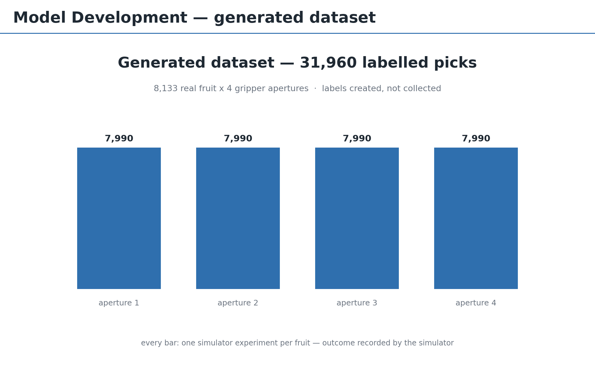
Figure 3. Generated dataset — 31,960 labelled picks. 8,133 real fruit × 4 gripper apertures. Labels created, not collected.
Four bars, all at 7,990. Each fruit contributes one pick to every aperture band, and the reason they are equal is the design rather than a coincidence.
The generator settles a fruit for 2,400 steps under gravity alone, saves that settled state, then tries all four apertures starting from the same saved state each time. The four rows that come out differ in the aperture and in nothing else.
That is a counterfactual structure, and it is why the aperture’s effect can be read causally. Observation cannot produce it. In a real orchard the same apple cannot be picked four times.
31,960 rows. Fifteen observations per row, all of them things a camera could supply: position, diameter, stalk direction, distance and bearing to neighbours, clearance along the approach. Nothing the simulator knows privately, such as internal stress or contact force, is used as an input. That constraint is what keeps the model portable to a real machine later.
Runs that diverged were removed at the fruit level rather than the row level. A palm two metres from where it should be, a pick past thirty seconds, four fingers in contact when there are three: those are not hard cases, they are numbers without physical meaning. Dropping one row would break the counterfactual structure for the other three, so the whole fruit goes. 143 of 8,133, or 1.8 per cent.
Two models, not one
Video 2. Two fruit propping each other up. The first comes away, and the survivor settles plumb because nothing is holding it any more.
Harvesting is not a sequence of independent events. Take one apple and the ones touching it move, and the pose they settle into changes the odds for the next pick. A planner that does not know this is planning on a tree that stopped existing after the first pick.
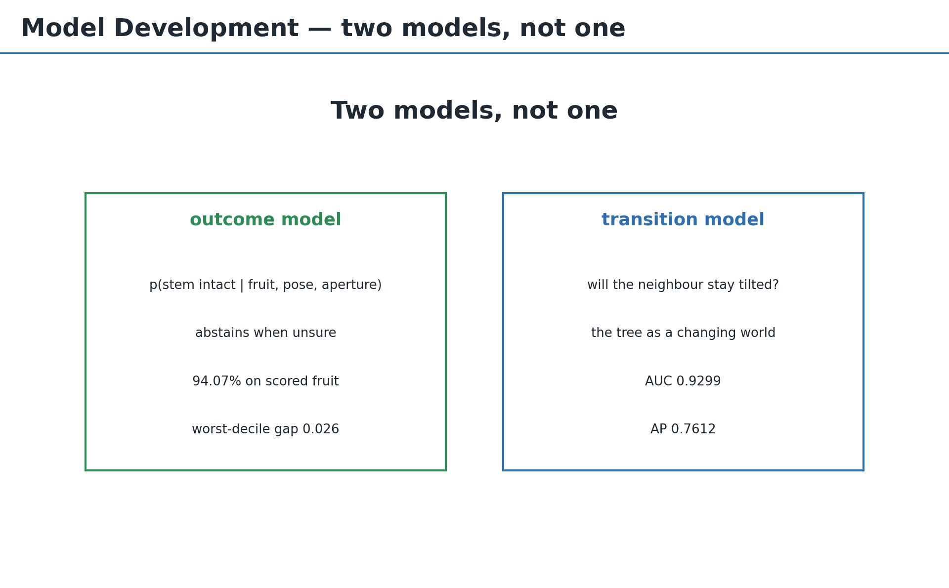
Figure 4. Two models, not one. The outcome model predicts whether the stem survives a pick. The transition model asks what happens to the tree after each pick — the tree as a changing world.
So there are two. The outcome model predicts six classes for a pick: stem intact, neighbour knocked, stalk damage, grasp failed, no corridor, not detached. It reaches 94.07 per cent on held-out fruit with a worst-decile calibration gap of 0.026, and it abstains rather than guessing when unsure.
The transition model answers a narrower question: given a pick and its neighbours, will each neighbour still be tilted once the scene settles?
What makes the second one interesting is how much of the problem physics removes before the model sees it.
| Situation | Outcome |
|---|---|
| Only one neighbour left supporting it | Always hangs plumb. No exception in 99 cases, mean tilt 0.004° |
| Two or more still in contact | The outcome divides. About 12% stay tilted |
Table 2. The transition model only judges the second row.
The first row is settled by gravity, not by learning. Handing it to the model would let an easy majority mask a hard minority and inflate the score. So the training set contains only the ambiguous cases, and the model reports AUC 0.9299 with AP 0.7612 on those.
Choosing the tools
Four choices, each with alternatives that were reasonable. The reasoning matters more than the names.
MuJoCo, not PyBullet or Isaac. Contact is solved analytically, so penetration does not accumulate when three fingers close on a fruit. It is deterministic, which is what makes a paired comparison valid at all: run the same seed twice and the numbers are identical to the bit. And scenes assemble from XML strings, which is what allows a different gripper per fruit. No GPU, no licence.
LightGBM for the outcome model, not a neural network. Fifteen tabular columns, six classes. Gradient boosting wins that shape of problem, and training in under a minute meant the canopy could be regenerated three times and the model refitted each time. Since the planner consumes the probabilities directly rather than the argmax, calibration stability mattered more than raw accuracy.
CatBoost for the transition model. Same tabular shape, different winner. Where AUC tied, CatBoost was better on average precision and Brier score, and it trained 53 times faster than the neural alternative. At a 12 per cent base rate AUC is insensitive, so AP and Brier decided it.
A Transformer for station selection. The input is a variable-length set with no meaningful order: fruit counts differ per tree, and shuffling the list must not change the answer. Padding an MLP breaks permutation invariance and a graph network needs its structure defined separately. Autoregressive decoding also gives something the others do not, which the next section explains.
None of these are novel architectures. The point was to show the data is learnable with standard ones.
The planner: five modules
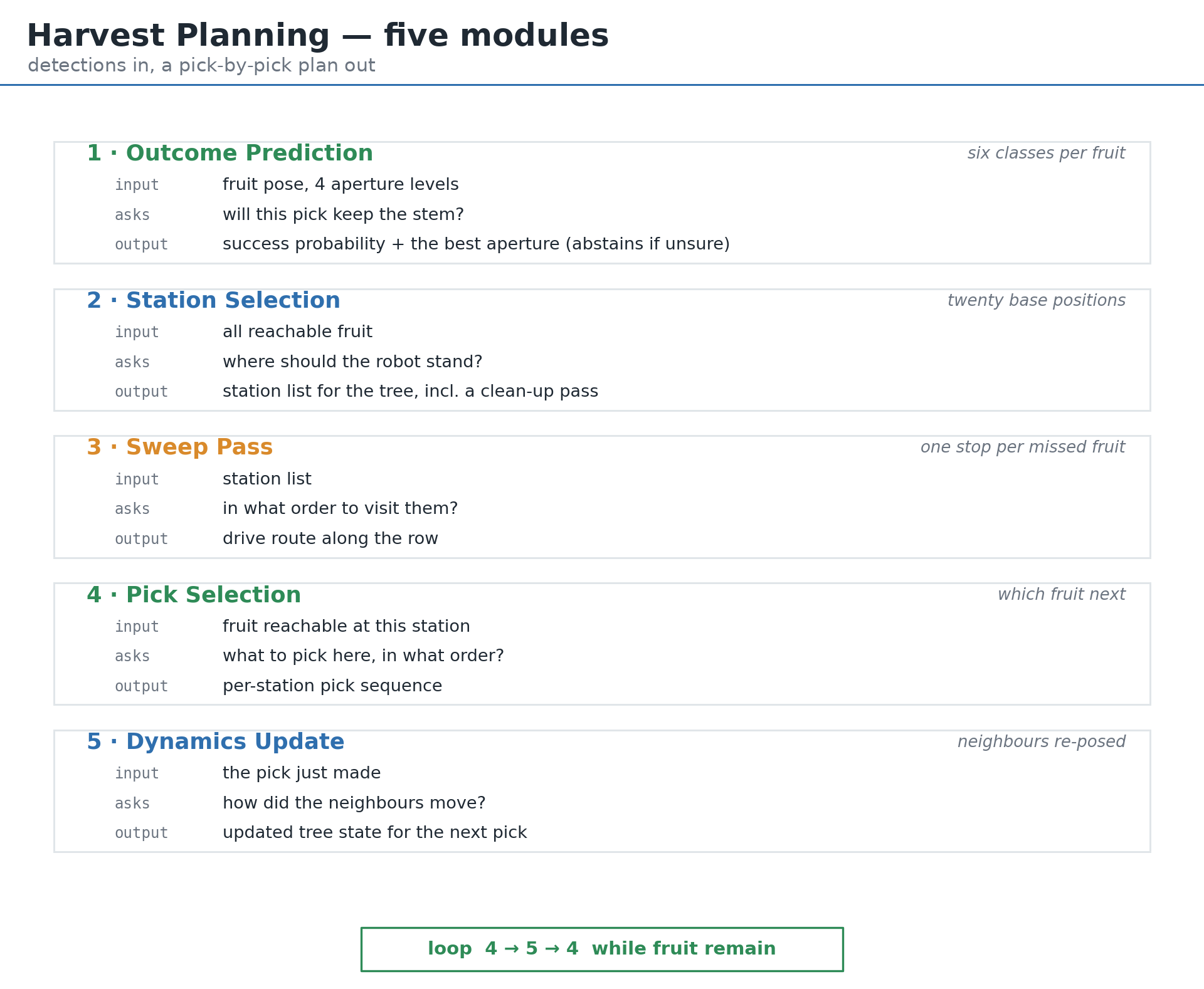
Figure 5. The five modules of the harvest planner. Steps 4 and 5 loop until no fruit remain.
With the models in place, a plan for one tree comes out of five steps.
1 · Outcome prediction. Every reachable fruit on the tree gets six probabilities.
2 · Station selection. Where should the base stop? A short arm reaches about nine fruit from any one position, which is why a single tree needs more than twenty stops. The learned planner picks twenty positions autoregressively, marking the fruit each one covers so the next choice sees only what remains. An earlier version scored all candidate positions at once and produced three stops within 15 cm of each other: individually good, collectively useless.
3 · Sweep pass. Some fruit are within the arm’s reach but visible only from a position that covers nothing else. A rule that stops when marginal gain hits zero walks straight past them. So one dedicated stop is added per missed fruit, 1.3 per tree on average, and that is what takes coverage of reachable fruit to 100 per cent.
4 · Pick selection. Which fruit now? The one with the highest expected utility.
5 · Dynamics update. After each pick, the neighbours are re-posed and the probabilities from step 1 are recomputed.
Steps 4 and 5 loop until nothing is left. That loop is why a plan is not a static list: the order changes the tree, and the tree changes what the next order should be.
What a person sees
A plan is a CSV. A grower cannot read a CSV and decide whether to trust it.
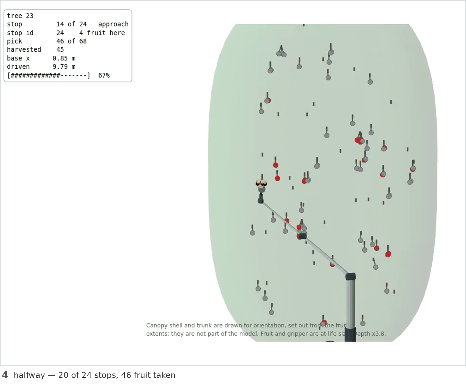
Figure 6. Plan playback, stop 14 of 24, 46 of 68 fruit harvested. Every pick is played back from the physics log, so what appears on screen cannot disagree with what was computed.
So there is an application layer on top of the planning module. It renders the canopy, drives the base from stop to stop, and plays every pick back from the physics log. Nothing is animated by hand, so what appears on screen cannot disagree with what was computed.
On paper a plan is “24 stops, 68 picks, 21.8 minutes.” On screen you can see whether the routing doubles back, whether coverage is even, and where the arm never reaches. That is what a grower would look at before letting a machine into a block.
Two more screens sit beside it. One profiles the incoming detections, because a plan built on a bad detection set is a bad plan and the failure is silent otherwise. The other breaks the result down: volume by grade, variation between trees, and where fruit is lost at each stage.
The separation is deliberate.
| What it does | How often it changes | |
|---|---|---|
| Planning module | Produces the plan | Rarely |
| Application layer | Lets a person understand and judge it | Differs per farm |
Table 3. Calculation and judgement are kept apart.
Changing one does not disturb the other. The planner can be improved without touching the screens, and the screens can be reshaped for a particular farm without putting the numbers at risk.
What one row looks like
It is worth seeing a single row before moving on, because the abstraction hides how concrete this is.
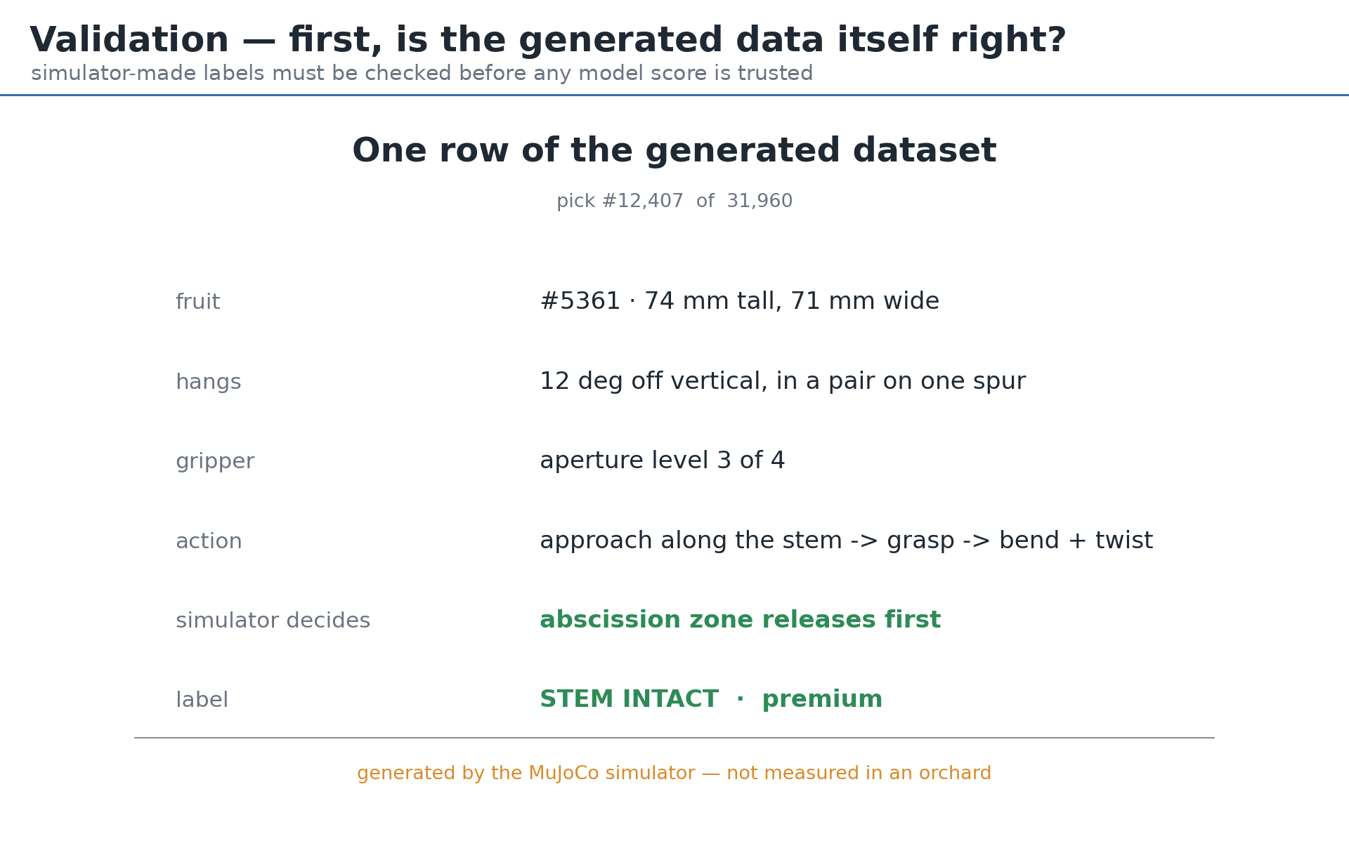
Figure 7. One row of the generated dataset. Generated by the simulator — not measured in an orchard.
pick #12,407 of 31,960

fruit              #5361 · 74 mm tall, 71 mm wide
hangs              12 deg off vertical, in a pair on one spur
gripper            aperture level 3 of 4
action             approach along the stem -> grasp -> bend + twist
simulator decides  abscission zone releases first
label              STEM INTACT · premium
Generated by the simulator. Not measured in an orchard. Every model in this project is trained on 31,960 rows of that, and the planner rests on the models.
Source, weights and derived data are public under MIT. github.com/isupernova-io/aipick-harvest-planner
Physics World Models — Building an End-to-End AI Harvest Planner
| Part 1 | Problem & Design | Where the Rules Are Known but the World Is Missing |
| Part 2 | Building the Model | From Physics to 31,960 Labelled Picks |
| Part 3 | Validation & What Comes Next | Grading Against the Simulator, Not the Model |